Project journal
Data Engineering
An end-to-end academic flood-monitoring project I developed myself, including ingestion, orchestration, warehouse processing, and the BI work built around the outputs.
- Where
- Mahidol University · ITDS344
- Project period
- Course project
- My role
- Sole developer · data pipeline and BI
Owning the path from incoming data to analysis
I developed this Data Engineering project myself, including the BI portion. The starting problem was that useful water and weather data existed across separate sources. I wanted to bring those inputs together in a province-level view, with a pipeline behind the dashboard that could explain where the information came from.
The project combines dam and reservoir observations from the Royal Irrigation Department, weather inputs, and historical flood-risk areas. The presentation frames water-management teams, warning centers, and insurers as intended users. My implementation connects ingestion, transformation, quality checks, warehouse tables, and Power BI reporting in one academic system.
What the pipeline feeds into
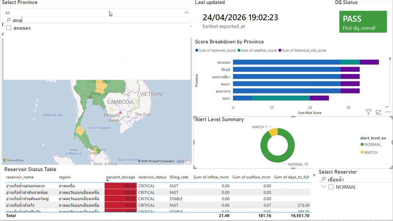
An original Power BI screenshot from the project presentation. It shows a recorded project snapshot, rather than live conditions.
 View full size ↗
Making the pipeline's responsibilities explicit
The dam and reservoir APIs feed Kafka and then HDFS Bronze, retaining raw observations before transforming them. The historical risk file is a static input, while weather enters through a separate path with a simulated fallback. Those sources have different update patterns, so ingestion and the scheduled analytical workflow have separate responsibilities.
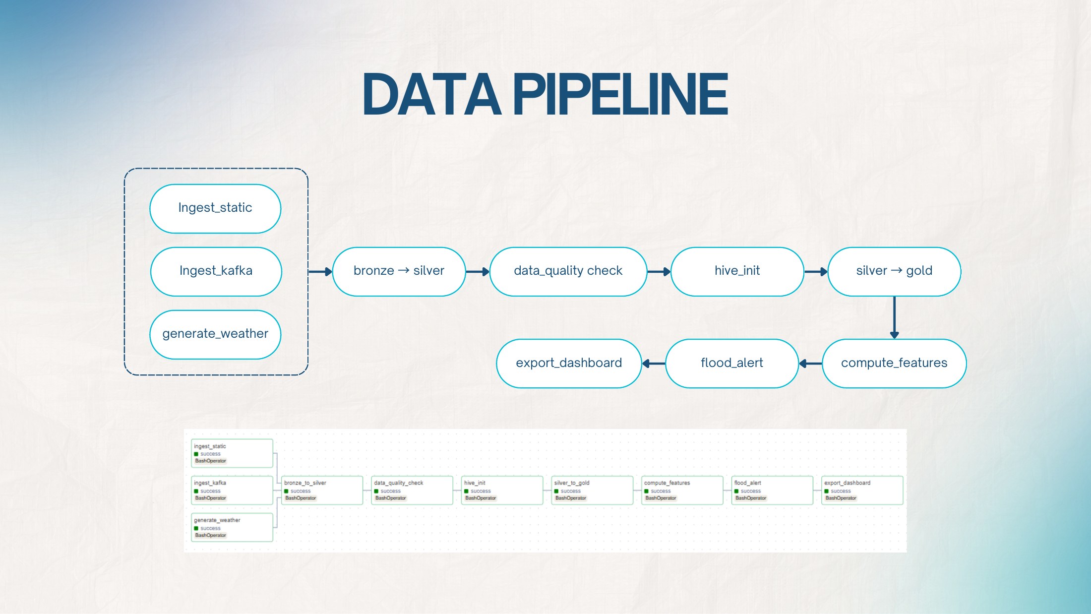
Airflow organizes the workflow on a six-hour schedule: ingest the inputs, transform Bronze into Silver, run quality checks, initialize Hive, build Gold tables, compute features and alert scores, then export for the dashboard. Keeping those stages explicit made it possible to follow a reporting value back through the processing steps that produced it.
Incremental ingestion instead of a blind reload
The reservoir producer calls the Royal Irrigation Department dam and reservoir endpoints and publishes normalized messages to a three-partition Kafka topic. On its first run it backfills seven historical days; later runs fetch the current observations plus the previous day's historical data. A producer state file records the latest historical date so that the backfill behavior is explicit rather than accidental.
The Kafka consumer maintains a separate fetched-at watermark and only writes records newer than that point. Bronze files are partitioned by source and date in HDFS, which makes reruns safer and gives the next stage a clear boundary between newly ingested data and records that have already been processed.
From raw files to a warehouse that can be rebuilt
The Bronze-to-Silver step uses pandas and PyArrow to cast types, standardize fields, handle nulls, deduplicate records, and write date-partitioned Parquet with Snappy compression. Reservoir, weather, and historical-risk datasets keep separate Silver paths because their schemas and refresh patterns are different.
Hive exposes the Silver datasets as external tables, then loads a Gold star schema with reservoir, location, and weather dimensions plus water-monitoring and flood-risk facts. The loaders use overwrite-based, partition-aware operations so the same date can be rebuilt without appending another copy. Docker Compose provides the local Kafka, HDFS/YARN, Hive, PostgreSQL, and Airflow services used to run that architecture together.
Following the work through Airflow
The pipeline diagram and Airflow task graph from the original presentation.
 View full size ↗
A dashboard is only useful if the inputs make sense
A large part of the work happened before the charts. I standardized numeric types, column names, and dates; trimmed strings; handled missing fields; and deduplicated observations using reservoir ID, date, and source. The transformation also recalculated storage percentage from volume and capacity to address inconsistencies in the incoming data.
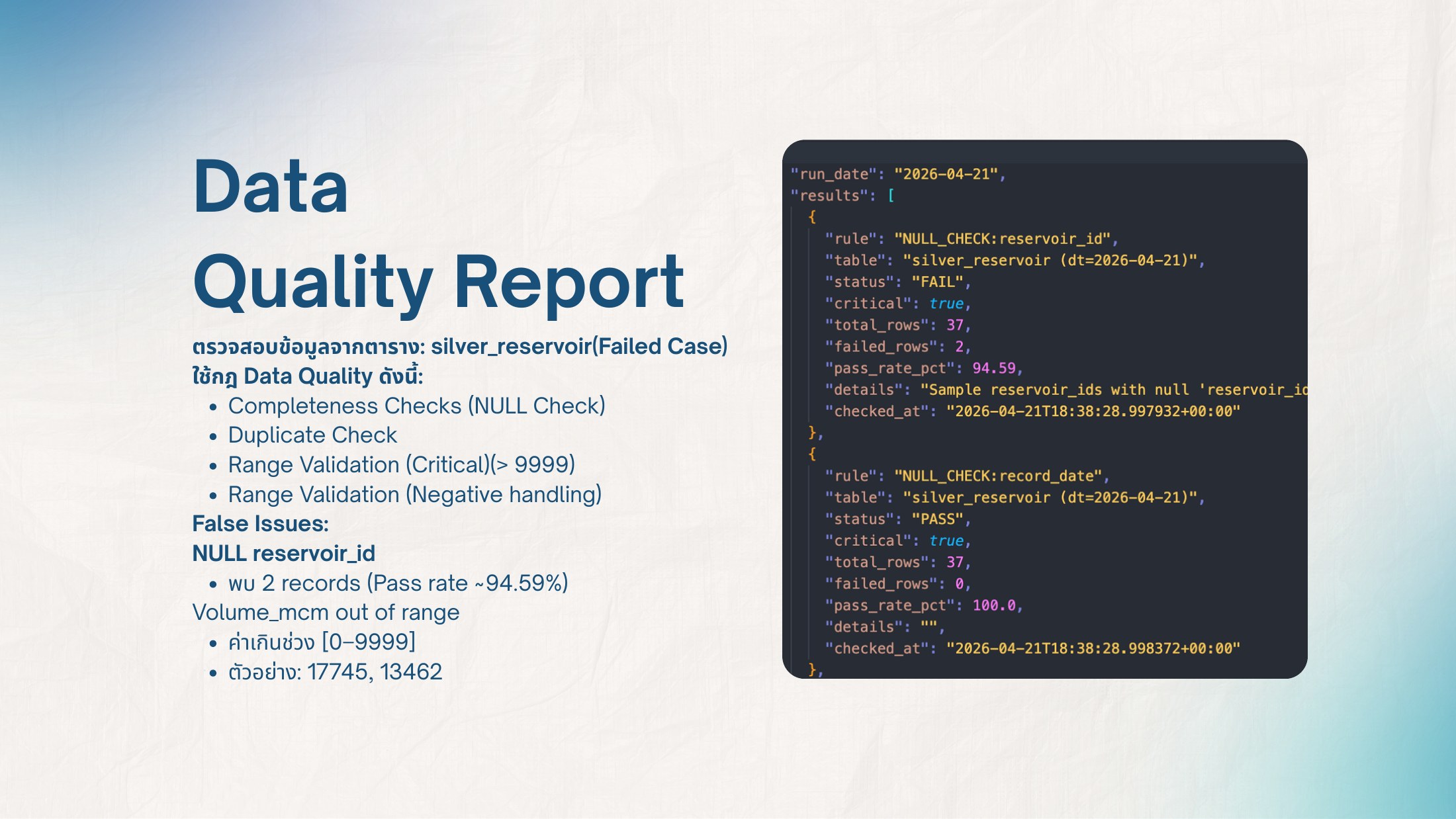
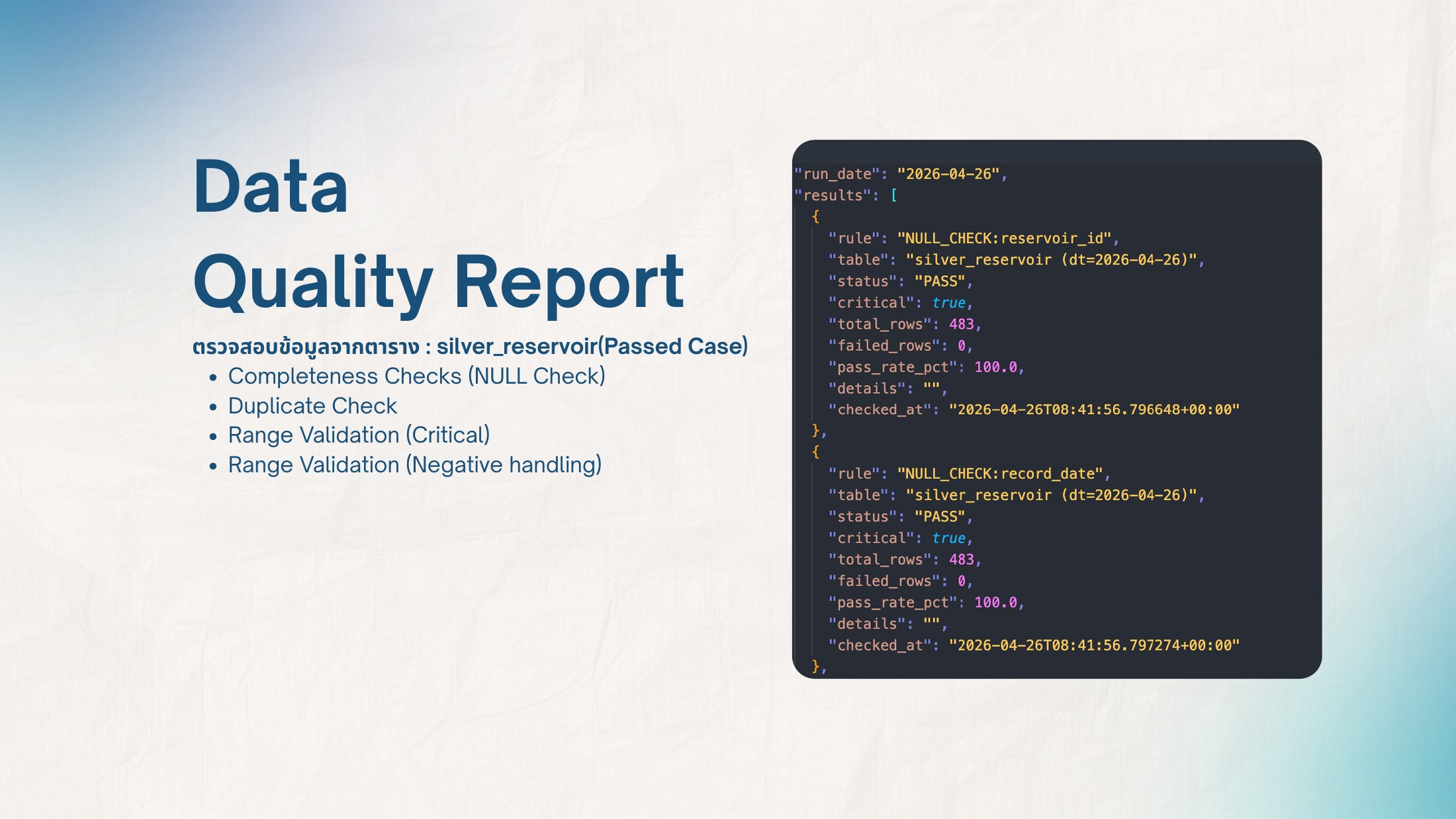
The quality checks looked for missing keys, duplicate records, and values outside the configured ranges. The presentation includes a failed run with missing reservoir IDs and out-of-range volumes, alongside a separate passing run. These checks gave me a concrete way to inspect what should be corrected or investigated before trusting the downstream analysis.
Making data-quality results visible
Two recorded examples from the project presentation. They use different dates and batches; they are not a before-and-after comparison of the same data.
 View full size ↗
 View full size ↗
Keeping derived risk features explainable
A seven-day window produces reservoir features such as net flow, one-day storage change, average storage trend, estimated days to full, reservoir status, and filling-rate category. The feature code keeps the thresholds visible—for example, storage at 90% or above is marked critical—so a dashboard label can be traced back to a concrete rule.
The province-level alert is also rule based. Reservoir conditions contribute up to 40 points, weather up to 35, and historical risk up to 25. Totals below 25 are normal, while 25, 50, and 75 mark watch, alert, and crisis thresholds. I present this logic as an inspectable coursework model, not as a statistically validated flood forecast.
The BI work is part of the same project
I also handled the business-intelligence side, using the exported reservoir information, province-level scores, and pipeline metadata. The Power BI view includes province and reservoir selectors, a map, a stacked breakdown of reservoir, weather, and historical-risk scores, an alert-level summary, and a reservoir status table.
I included the update timestamp and data-quality status alongside the charts so the report also exposed information about its inputs. The presentation includes a business-query example for looking at a dam's water-volume trend over the previous 30 days. Together, those pieces connect the engineering work to questions someone can explore in the reporting layer.